pacman::p_load(dplyr,tidyr,stringr,readr,fs,purrr,ggplot2, plotly, ggstatsplot,igraph,lubridate,hms, vcd)Task 1: Knowledge Mastery and Weak Links
1. Overview
NorthClass, a prominent higher education institution with over 300,000 registered learners, offers more than 100 courses across various disciplines. To enhance its digital age competitiveness, NorthClass launched a programming course requiring learners to complete tasks with multiple submissions. Post-course, the institution collects learning data to assess instructional quality. NorthClass plans to form a Smart Education Development and Innovation Group to leverage AI for improving education and nurturing innovative talents. Visualization and Visual Analytics are proposed to transform complex learning data into intuitive graphical representations, aiding in diagnosing knowledge mastery, monitoring learning trends, and identifying factors causing learning difficulties. The task is to design and implement a Visual Analytics solution to help NorthClass perceive learners’ progress and provide recommendations for teaching strategy adjustments and course design improvements.
2. Our Task
From the Challenge, the key problem statement was to perform a comprehensive analysis of multiple datasets that describe various aspects of the learner’s profile, learning patterns and status, to derive key insights to enhance teaching strategies and course design.
Consequently the key requirements based on the 5 stipulated tasks in the challenge were as follows.
Task 1: To provide a quantitative assessment of the learners’ knowledge mastery and identify weak links in their knowledge system, based on the multi-dimensional attributes such as answer scores and answer status in the learners’ log records of the learners’ question-answering behaviors.
This would entail an analysis of the learners’ aggregate performance in their programming tasks (a.k.a. questions in the dataset), including measures of central tendency, or any notable patterns that can glean insights towards knowledge mastery and weaknesses from the given datasets.
3. The Datasets
The provided materials for the challenge include 3 datasets described below, as well as a separate document providing a more detailed description of the data and variables
Dataset 1: Student Information - This comprises of 5 Cols, 1364 Rows, providing individualised demographic variables of the learners (a.k.a students) within the scope this project
Dataset 2: Learning Subject Title Information - This comprises of 5 Cols, 44 Rows, providing variables of the questions from the programming tasks which are collated in the scope of this project
Dataset 3: Class Submission Records - This comprises of multiple datasets, each with 10 Cols and various number of rows, providing supposedly the participating learners’ answering variables to the questions collated in the scope of this project
4. Methodology
Our methodology systematically integrates data collection, data processing, analysis, pattern mining, modeling, and recommendations to create a comprehensive Visual Analytics solution for improving teaching strategies and course designs at NorthClass Institute, showing as below: 
5. Getting Started
5.1 Loading R packages
The code chunk below imports the dataset into R environment by using read_csv() function of readr package. readr is one of the tidyverse package.
Read the individual CSV files into data frames. Check that the structure of each data frame is the same.
5.2 Importing data
The code chunk below imports the dataset into R environment by using read_csv() function of readr package. readr is one of the tidyverse package.
Read the individual CSV files into data frames. Check that the structure of each data frame is the same.
df_StudentInfo <- read_csv("data/Data_StudentInfo.csv")
df_TitleInfo <- read_csv("data/Data_TitleInfo.csv")
csv_file_list <- dir('data/Data_SubmitRecord')
csv_file_list <- paste0("./data/Data_SubmitRecord/",csv_file_list)
df_StudentRecord <- NULL
for (file in csv_file_list) { # for every file...
file <- read_csv(file)
df_StudentRecord <- rbind(df_StudentRecord, file) # then stick together by rows
}
df_StudentRecord %>% glimpse()Rows: 232,818
Columns: 10
$ index <dbl> 0, 1, 2, 3, 4, 5, 6, 7, 8, 9, 10, 11, 12, 13, 14, 15, 16, …
$ class <chr> "Class1", "Class1", "Class1", "Class1", "Class1", "Class1"…
$ time <dbl> 1704209872, 1704209852, 1704209838, 1704208923, 1704208359…
$ state <chr> "Absolutely_Correct", "Absolutely_Correct", "Absolutely_Co…
$ score <dbl> 3, 3, 3, 3, 4, 0, 3, 3, 3, 3, 3, 3, 3, 1, 3, 1, 1, 4, 0, 0…
$ title_ID <chr> "Question_bumGRTJ0c8p4v5D6eHZa", "Question_62XbhBvJ8NUSnAp…
$ method <chr> "Method_Cj9Ya2R7fZd6xs1q5mNQ", "Method_gj1NLb4Jn7URf9K2kQP…
$ memory <dbl> 320, 356, 196, 308, 320, 0, 308, 312, 312, 328, 512, 324, …
$ timeconsume <chr> "3", "3", "2", "2", "3", "5", "2", "2", "3", "2", "3", "2"…
$ student_ID <chr> "8b6d1125760bd3939b6e", "8b6d1125760bd3939b6e", "8b6d11257…5.3 Data Preparation
5.3.1 Check Missing Values
First, we identify students who are enrolled in more than one class. This helps us focus on those who need their class assignments reviewed. For students enrolled in multiple classes, we determine the correct class by identifying which class they attended most frequently. Finally, we update the class assignments in the original dataset. We replace the incorrect class values with the correct class determined in the previous step. This ensures that each student is associated with the class they attended most often. #### Missing Data
colSums() and is.NA() functions are used to search for missing values as a whole for the 3 data sets in the code chunks as follows.
#Find the number of missing values for each col
colSums(is.na(df_StudentInfo))
index student_ID sex age major
0 0 0 0 0 #Find the number of missing values for each col
colSums(is.na(df_TitleInfo)) index title_ID score knowledge sub_knowledge
0 0 0 0 0 #Find the number of missing values for each col
colSums(is.na(df_StudentRecord)) index class time state score title_ID
0 0 0 0 0 0
method memory timeconsume student_ID
0 0 0 0 Click to show code
Check for duplicate rows
Using duplicated(), duplicate rows in each of the 3 data sets are identified and extracted in the following code chunks.
df_StudentInfo[duplicated(df_StudentInfo), ]# A tibble: 0 × 5
# ℹ 5 variables: index <dbl>, student_ID <chr>, sex <chr>, age <dbl>,
# major <chr>df_TitleInfo[duplicated(df_TitleInfo), ]# A tibble: 0 × 5
# ℹ 5 variables: index <dbl>, title_ID <chr>, score <dbl>, knowledge <chr>,
# sub_knowledge <chr>df_StudentRecord[duplicated(df_StudentRecord), ]# A tibble: 0 × 10
# ℹ 10 variables: index <dbl>, class <chr>, time <dbl>, state <chr>,
# score <dbl>, title_ID <chr>, method <chr>, memory <dbl>, timeconsume <chr>,
# student_ID <chr>From the outputs above, there were no duplicate rows found.
Data Wrangling for Inconsistencies
To get a better understanding of the variables in the original dataset, the glimpse() function is used in the following code chunks.
glimpse(df_StudentInfo)Rows: 1,364
Columns: 5
$ index <dbl> 1, 2, 3, 4, 5, 6, 7, 8, 9, 10, 11, 12, 13, 14, 15, 16, 17, …
$ student_ID <chr> "8b6d1125760bd3939b6e", "63eef37311aaac915a45", "5d89810b20…
$ sex <chr> "female", "female", "female", "female", "male", "male", "ma…
$ age <dbl> 24, 21, 23, 21, 22, 19, 21, 18, 21, 24, 23, 20, 18, 18, 23,…
$ major <chr> "J23517", "J87654", "J87654", "J78901", "J40192", "J57489",…Identifying Other Unexpected Duplicate Values
Considering intuitively unique values for certain variables or dependent variables, other forms of duplicates are also identified and cleaned where relevant.
- Duplicate student_ID in StudentInfo
# Find the duplicated student_IDs
duplicates <- df_StudentInfo[duplicated(df_StudentInfo$student_ID) | duplicated(df_StudentInfo$student_ID, fromLast = TRUE), ]

# Display the rows with duplicate student_IDs
duplicates
# A tibble: 0 × 5
# ℹ 5 variables: index <dbl>, student_ID <chr>, sex <chr>, age <dbl>,
# major <chr>From the output above, no duplicates found.
- Duplicate title_ID (aka questions) in TitleInfo
# Find the duplicated title_IDs
duplicates <- df_TitleInfo[duplicated(df_TitleInfo$title_ID) | duplicated(df_TitleInfo$title_ID, fromLast = TRUE), ]

# Display the rows with duplicate title_IDs
duplicates
# A tibble: 12 × 5
index title_ID score knowledge sub_knowledge
<dbl> <chr> <dbl> <chr> <chr>
1 2 Question_q7OpB2zCMmW9wS8uNt3H 1 r8S3g r8S3g_n0m9rsw4
2 3 Question_q7OpB2zCMmW9wS8uNt3H 1 r8S3g r8S3g_l0p5viby
3 21 Question_QRm48lXxzdP7Tn1WgNOf 3 y9W5d y9W5d_c0w4mj5h
4 22 Question_QRm48lXxzdP7Tn1WgNOf 3 m3D1v m3D1v_r1d7fr3l
5 23 Question_pVKXjZn0BkSwYcsa7C31 3 y9W5d y9W5d_c0w4mj5h
6 24 Question_pVKXjZn0BkSwYcsa7C31 3 m3D1v m3D1v_r1d7fr3l
7 26 Question_lU2wvHSZq7m43xiVroBc 3 y9W5d y9W5d_c0w4mj5h
8 27 Question_lU2wvHSZq7m43xiVroBc 3 k4W1c k4W1c_h5r6nux7
9 30 Question_x2Fy7rZ3SwYl9jMQkpOD 3 y9W5d y9W5d_c0w4mj5h
10 31 Question_x2Fy7rZ3SwYl9jMQkpOD 3 s8Y2f s8Y2f_v4x8by9j
11 36 Question_oCjnFLbIs4Uxwek9rBpu 3 g7R2j g7R2j_e0v1yls8
12 37 Question_oCjnFLbIs4Uxwek9rBpu 3 m3D1v m3D1v_r1d7fr3lunique(duplicates$knowledge)[1] "r8S3g" "y9W5d" "m3D1v" "k4W1c" "s8Y2f" "g7R2j"unique(duplicates$sub_knowledge)[1] "r8S3g_n0m9rsw4" "r8S3g_l0p5viby" "y9W5d_c0w4mj5h" "m3D1v_r1d7fr3l"
[5] "k4W1c_h5r6nux7" "s8Y2f_v4x8by9j" "g7R2j_e0v1yls8"unique(df_TitleInfo$knowledge)[1] "r8S3g" "t5V9e" "m3D1v" "y9W5d" "k4W1c" "s8Y2f" "g7R2j" "b3C9s"unique(df_TitleInfo$sub_knowledge) [1] "r8S3g_l0p5viby" "r8S3g_n0m9rsw4" "t5V9e_e1k6cixp" "m3D1v_r1d7fr3l"
[5] "m3D1v_v3d9is1x" "m3D1v_t0v5ts9h" "y9W5d_c0w4mj5h" "k4W1c_h5r6nux7"
[9] "s8Y2f_v4x8by9j" "y9W5d_p8g6dgtv" "y9W5d_e2j7p95s" "g7R2j_e0v1yls8"
[13] "g7R2j_j1g8gd3v" "b3C9s_l4z6od7y" "b3C9s_j0v1yls8"Based on the output above, there is a total of 8 knowledge areas and 15 sub-knowledge areas. This suggests that majority of the knowledge areas and approximately half of sub-knowledge areas have overlapping title_ID. From the nomenclature, each sub-knowledge area is tagged to only 1 knowledge area.
To meaningfully analyse the relationship between knowledge areas & sub knowledge areas and other variables, additional columns are introduced where the values in these 2 columns are transposed as column labels with binary values to indicate the tagging of each question to that value. This is done in the following code chunk. 3. Duplicate class for each Individual Students in StudentRecord
# Identify students with multiple classes
students_multiple_classes <- df_StudentRecord %>%
  group_by(student_ID) %>%
  summarise(unique_classes = n_distinct(class)) %>%
  filter(unique_classes > 1)

students_multiple_classes_entries <- df_StudentRecord %>%
  filter(student_ID %in% students_multiple_classes$student_ID) %>%
  group_by(student_ID, class) %>%
  summarise(count = n()) %>%
  arrange(desc(count)) %>%
  arrange(desc(student_ID))

# Display the results
print(students_multiple_classes_entries)
# A tibble: 12 × 3
# Groups: student_ID [6]
student_ID class count
<chr> <chr> <int>
1 r9m46ndmmmzeeehft96z Class15 140
2 r9m46ndmmmzeeehft96z class 1
3 qz6jjynwbd3szlp0rj04 Class1 136
4 qz6jjynwbd3szlp0rj04 class 1
5 nd9xpohv0s4ttw0o7fts Class8 143
6 nd9xpohv0s4ttw0o7fts class 1
7 lqm8jh0uggps7yd0lx2x Class8 132
8 lqm8jh0uggps7yd0lx2x class 1
9 isa355t9q5rut5fm8aml Class1 142
10 isa355t9q5rut5fm8aml class 1
11 ezdogkk0jqt4nvvvbnxp Class7 125
12 ezdogkk0jqt4nvvvbnxp class 1Based on the output above, it is apparent that the 2nd class for each of the student above is an erroneous value. Hence this inconsistency will be cleaned in the following code chunk
# Step 1: Identify the correct class for each student (the class with the highest frequency)
correct_classes <- df_StudentRecord %>%
  filter(student_ID %in% students_multiple_classes$student_ID) %>%
  group_by(student_ID, class) %>%
  summarise(count = n()) %>%
  arrange(desc(count)) %>%
  slice(1) %>%
  select(student_ID, correct_class = class)

# Step 2: Replace wrong class values
df_StudentRecord <- df_StudentRecord %>%
  left_join(correct_classes, by = "student_ID") %>%
  mutate(class = ifelse(!is.na(correct_class), correct_class, class)) %>%
  select(-correct_class)
For completeness, a check is done for existence of other students with class that has no class number in the following code chunk.
MissingClassNo <- df_StudentRecord %>%
  filter(class == "class")
MissingClassNo
# A tibble: 0 × 10
# ℹ 10 variables: index <dbl>, class <chr>, time <dbl>, state <chr>,
# score <dbl>, title_ID <chr>, method <chr>, memory <dbl>, timeconsume <chr>,
# student_ID <chr>Based on the output above, there are no further students with class without number.
Identifying Other Unexpected and/or Missing Values
- Missing Student_ID and title_ID in StudentRecord are also identified.
missing_students <- anti_join(df_StudentRecord, df_StudentInfo, by = "student_ID")

# Display the missing student IDs
missing_student_ids <- missing_students %>% select(student_ID) %>% distinct()
print(missing_student_ids)
# A tibble: 1 × 1
student_ID
<chr>
1 44c7cf3881ae07f7fb3eDmissing_questions <- anti_join(df_StudentRecord, df_TitleInfo, by = "title_ID")
# Display the missing title IDs
missing_questions <- missing_questions %>% select(title_ID) %>% distinct()
print(missing_questions)# A tibble: 0 × 1
# ℹ 1 variable: title_ID <chr>There is 1 missing student between either StudentRecord or StudentInfo, but no missing questions. Since there is partial missing info on this student, it isn’t meaningful to include in this analysis, hence the student_ID will be excluded in the following code chunk.
df_StudentInfo <- df_StudentInfo %>%
  filter (student_ID != '44c7cf3881ae07f7fb3eD')
df_StudentRecord <- df_StudentRecord %>%
filter (student_ID != '44c7cf3881ae07f7fb3eD')- Other unexpected values
The unique values for each column is queried to check for unexpected values in the following code chunk, wherein Index, time, class, title_ID and student_ID are excluded since they will be dealt with separately
unique(df_StudentRecord$state) [1] "Absolutely_Correct" "Error1" "Absolutely_Error"
[4] "Error6" "Error4" "Partially_Correct"
[7] "Error2" "Error3" "Error5"
[10] "Error7" "Error8" "Error9"
[13] "�������" unique(df_StudentRecord$score)[1] 3 4 0 1 2unique(df_StudentRecord$method)[1] "Method_Cj9Ya2R7fZd6xs1q5mNQ" "Method_gj1NLb4Jn7URf9K2kQPd"
[3] "Method_5Q4KoXthUuYz3bvrTDFm" "Method_m8vwGkEZc3TSW2xqYUoR"
[5] "Method_BXr9AIsPQhwNvyGdZL57"unique(df_StudentRecord$memory) [1] 320 356 196 308 0 312 328 512 324 188 316 344
[13] 444 192 332 484 360 200 340 184 476 492 180 448
[25] 464 8544 204 496 364 460 508 456 352 480 348 488
[37] 468 400 616 472 384 376 452 336 588 604 440 600
[49] 580 500 640 520 436 368 612 504 736 632 8448 220
[61] 372 208 828 256 568 576 628 756 620 700 212 592
[73] 380 396 432 404 644 564 748 216 264 708 768 304
[85] 420 624 8516 8644 288 8632 8640 8512 408 260 292 608
[97] 8580 636 536 424 596 272 388 300 280 268 176 160
[109] 296 416 240 284 248 172 8388 832 4164 4284 428 168
[121] 572 164 276 528 392 412 8668 8500 8540 8664 8536 8576
[133] 8628 8504 8800 8524 8392 8548 692 952 8508 8648 9664 9536
[145] 9564 49852 59616 1332 948 824 724 2876 3024 24668 25208 26712
[157] 23968 732 25248 22740 712 8520 720 18264 224 4984 8696 20272
[169] 19576 516 8976 9028 9532 544 584 552 524 5624 29688 688
[181] 30940 44020 740 556 51376 14656 65536 680 30440 30284 23128 28112
[193] 760 15060 25660 23356 31796 804 24768 24232 12792 14720 26172 29020
[205] 32992 28492 10568 8460 8404 908 652 540 8620 34268 11348 11640
[217] 13124 532 12608 15028 1400 32544 39612 27272 28852 29248 8452 8616
[229] 8480 8528 560 13576 8436 548 2012 24896 232 21728 21148 4424
[241] 7640 43512 39912 19936 12580 2412 2436 24224 4296 4332 6392 25912
[253] 21332 20128 668 35948 2360 8612 8384 5560 26548 25532 13112 15288
[265] 13992 49336 53216 15040 13780 8496 8424 37184 8476 8400 8408 30656
[277] 8156 8140 8064 8136 11236 5616 8160 4192 23116 19784 22908 21176
[289] 18276 20708 19868 16348 18716 17208 19588 14824 20780 20204 24932 21084
[301] 24992 21884 18764 26624 24368 13240 22988 3740 43532 26084 26320 13340
[313] 11372 46460 49464 13356 8144 8564 1720 13892 14488 10580 23576 8396
[325] 15212 15340 872 25648 25920 27028 24356 23544 7416 6560 4852 8556
[337] 32088 32716 44216 4292 228 33212 33736 27228 27288 11764 10540 11560
[349] 10456 11384 10708 32932 25940 17800 16764 46908 30512 9368 9472 19156
[361] 2348 36136 8132 4708 39048 21152 30632 27200 656 252 47096 8552
[373] 8464 14040 36984 2384 1792 6084 5844 2456 2440 26452 27364 648
[385] 244 23168 24324 8420 41460 40568 34316 896 1472 7156 23740 6444
[397] 6972 6200 6060 7488 6700 6580 5184 4948 5052 5820 6120 5404
[409] 5028 5180 5100 5068 5020 5204 5976 5176 5048 5884 5824 5828
[421] 5060 5072 5056 6076 6328 5076 8492 8428 236 7340 6668 7492
[433] 8412 8652 17176 6852 6616 6032 45288 50140 40348 16848 21820 20856
[445] 26296 28128 31560 17272 17656 37548 34476 38428 30456 41624 34224 18148
[457] 20816 128 808 156 844 728 716 696 836 676 4324 860
[469] 1980 8812 660 8636 684 8756 704 8532 8572 1920 1972 2332
[481] 2172 2296 2280 13908 63088 15432 15680 15624 15824 15956 15724 15292
[493] 8796 1880 1996 1992 11256 11268 11264 29240 29144 28752 27988 6068
[505] 1180 28536 11032 39216 35632 28600 2104 8656 36028 38432 12456 30164
[517] 1268 1328 1316 1240 50220 4540 35888 1976 4440 14336 14384 45680
[529] 39080 28484 39104 53732 8680 8692 8660 14136 4564 4480 28848 29112
[541] 18856 8792 8600 8592 41404 37052 36532 37804 33084 37368 30820 50620
[553] 26248 22264 26616 25900 752 47040 14644 40636 43128 33568 36248 33088
[565] 28140 28084 30532 30572 48376 47640 17400 20288 28724 20216 12664 12204
[577] 11960 27188 15700 15664 4580 4584 28036 28732 34004 33508 31808 1528
[589] 1716 13752 9592 9520 9784 9208 8828 28716 27536 28584 1704 1620
[601] 13096 14132 14584 57528 45500 7096 2168 2236 12984 20412 31172 29296
[613] 54356 54336 47548 41664 41812 13624 1336 1348 13496 55524 1352 1356
[625] 42052 744 996 984 940 1016 29012 28080 26036 7344 7232 7476
[637] 7828 13956 43452 1456 1324 1364 43196 27964 10812 972 1340 4692
[649] 27248 44592 44860 46576 20464 52656 52996 48964 49516 6904 6592 6584
[661] 8672 46852 40364 14500 14712 17740 17620 52584 8488 36488 44204 44500
[673] 42300 45228 17980 37460 28240 28988 53288 58424 9540 9524 6936 6204
[685] 54596 28604 29528 42804 12856 13776 15720 4156 12472 8704 8688 29300
[697] 18612 12976 32376 8776 13548 26456 1884 1752 764 4172 53316 52160
[709] 47036 45632 53396 51320 12468 11496 53604unique(df_StudentRecord$timeconsume) [1] "3" "2" "5" "4" "1" "9" "6" "--" "18" "61" "7" "59"
[13] "10" "8" "12" "13" "16" "15" "183" "68" "314" "64" "60" "11"
[25] "96" "94" "58" "67" "54" "17" "122" "19" "126" "14" "91" "50"
[37] "21" "40" "23" "20" "80" "31" "118" "400" "63" "25" "27" "29"
[49] "24" "26" "62" "152" "39" "22" "117" "30" "28" "48" "309" "331"
[61] "36" "65" "47" "46" "45" "52" "32" "42" "34" "38" "187" "37"
[73] "190" "163" "41" "53" "51" "307" "201" "184" "44" "43" "109" "33"
[85] "66" "326" "73" "49" "77" "82" "70" "71" "81" "35" "57" "75"
[97] "394" "385" "164" "78" "220" "217" "115" "86" "72" "88" "76" "134"
[109] "55" "84" "56" "106" "166" "124" "373" "289" "-" "135" "103" "114"
[121] "258" "254" "85" "69" "90" "132" "173" "272" "113" "116" "215" "123"
[133] "246" "146" "89" "245" "285" "205" "162" "165" "266" "172" "143" "377"
[145] "160" "159" "182" "74" "264" "153" "83" "286" "275" "280" "274" "269"
[157] "288" "271" "136" "276" "277" "356" "79" "147" "350" "315" "321" "302"unique(df_StudentInfo$sex)[1] "female" "male" unique(df_StudentInfo$age)[1] 24 21 23 22 19 18 20unique(df_StudentInfo$major)[1] "J23517" "J87654" "J78901" "J40192" "J57489"unique(df_TitleInfo$score)[1] 1 2 3 4unique(df_TitleInfo$knowledge)[1] "r8S3g" "t5V9e" "m3D1v" "y9W5d" "k4W1c" "s8Y2f" "g7R2j" "b3C9s"unique(df_TitleInfo$sub_knowledge) [1] "r8S3g_l0p5viby" "r8S3g_n0m9rsw4" "t5V9e_e1k6cixp" "m3D1v_r1d7fr3l"
[5] "m3D1v_v3d9is1x" "m3D1v_t0v5ts9h" "y9W5d_c0w4mj5h" "k4W1c_h5r6nux7"
[9] "s8Y2f_v4x8by9j" "y9W5d_p8g6dgtv" "y9W5d_e2j7p95s" "g7R2j_e0v1yls8"
[13] "g7R2j_j1g8gd3v" "b3C9s_l4z6od7y" "b3C9s_j0v1yls8"From the outputs above, there is an unexpected value for state and timeconsume in StudentRecord.
Starting with state, the rows with unexpected value(s) are queried in the following code chunk to better understand the number of affected rows.
Outlier_state <- df_StudentRecord %>%
  filter (state == '�������')
Outlier_state
# A tibble: 6 × 10
index class time state score title_ID method memory timeconsume student_ID
<dbl> <chr> <dbl> <chr> <dbl> <chr> <chr> <dbl> <chr> <chr>
1 6344 Class10 1.70e9 ����… 0 Questio… Metho… 65536 309 c681117f7…
2 6346 Class10 1.70e9 ����… 0 Questio… Metho… 65536 331 c681117f7…
3 6347 Class10 1.70e9 ����… 0 Questio… Metho… 65536 331 c681117f7…
4 10138 Class8 1.69e9 ����… 0 Questio… Metho… 65536 356 1883af270…
5 16420 Class8 1.69e9 ����… 0 Questio… Metho… 65536 356 hpb03ydul…
6 16458 Class8 1.69e9 ����… 0 Questio… Metho… 65536 356 ljylby8in…From the output above, there are only 6 rows that are affected. Further cross-validation with the data description document found that there should only be 12 unique values for this variable, and including this outlier state value will give 13. Hence this is likely a wrong entry, and so it will be excluded from the analysis in the following code chunk.
df_StudentRecord <- df_StudentRecord %>%
  filter (state != '�������')
For timeconsume, the rows with unexpected value(s) are queried in the following code chunk to better understand the number of affected rows.
Outlier_timeconsume <- df_StudentRecord %>%
  filter (timeconsume %in% c('-', '--'))
Outlier_timeconsume
# A tibble: 2,612 × 10
index class time state score title_ID method memory timeconsume student_ID
<dbl> <chr> <dbl> <chr> <dbl> <chr> <chr> <dbl> <chr> <chr>
1 191 Class1 1.70e9 Erro… 0 Questio… Metho… 0 -- 9417c1b4c…
2 321 Class1 1.70e9 Erro… 0 Questio… Metho… 0 -- 8b1fbc973…
3 322 Class1 1.70e9 Erro… 0 Questio… Metho… 0 -- 8b1fbc973…
4 366 Class1 1.70e9 Erro… 0 Questio… Metho… 0 -- 9ea29e4a7…
5 396 Class1 1.70e9 Erro… 0 Questio… Metho… 0 -- 9ea29e4a7…
6 397 Class1 1.70e9 Erro… 0 Questio… Metho… 0 -- 9ea29e4a7…
7 422 Class1 1.70e9 Erro… 0 Questio… Metho… 0 -- f06c3ddb1…
8 423 Class1 1.70e9 Erro… 0 Questio… Metho… 0 -- f06c3ddb1…
9 424 Class1 1.70e9 Erro… 0 Questio… Metho… 0 -- f06c3ddb1…
10 425 Class1 1.70e9 Erro… 0 Questio… Metho… 0 -- f06c3ddb1…
# ℹ 2,602 more rowsBased on the output, there is a sizable number of 2,612 rows with the unexpected value. Hence these rows will be kept in the analysis and replaced with 0 (since there is no existing values of 0 too), however subsequent analysis in this exercise involving the timeconsume variable will note these values as missing values. This is done in the following code chunk
df_StudentRecord <- df_StudentRecord %>%
  mutate(timeconsume = ifelse(timeconsume %in% c("-", "--"), 0, timeconsume))
unique(df_StudentRecord$timeconsume)
[1] "3" "2" "5" "4" "1" "9" "6" "0" "18" "61" "7" "59"
[13] "10" "8" "12" "13" "16" "15" "183" "68" "314" "64" "60" "11"
[25] "96" "94" "58" "67" "54" "17" "122" "19" "126" "14" "91" "50"
[37] "21" "40" "23" "20" "80" "31" "118" "400" "63" "25" "27" "29"
[49] "24" "26" "62" "152" "39" "22" "117" "30" "28" "48" "36" "65"
[61] "47" "46" "45" "52" "32" "42" "34" "38" "187" "37" "190" "163"
[73] "41" "53" "51" "307" "201" "184" "44" "43" "109" "33" "66" "326"
[85] "73" "49" "77" "82" "70" "71" "81" "35" "57" "75" "394" "385"
[97] "164" "78" "220" "217" "115" "86" "72" "88" "76" "134" "55" "84"
[109] "56" "106" "166" "124" "373" "289" "135" "103" "114" "258" "254" "85"
[121] "69" "90" "132" "173" "272" "113" "116" "215" "123" "246" "146" "89"
[133] "245" "285" "205" "162" "165" "266" "172" "143" "377" "160" "159" "182"
[145] "74" "264" "153" "83" "286" "275" "331" "280" "274" "269" "288" "271"
[157] "136" "276" "277" "79" "147" "350" "315" "321" "302"Removing Index Col
Each data set contains an index column, which is possibly to keep track of the original order and the total number of rows. This is no longer required and relevant in the analysis, hence it will be excluded.
#remove index column
df_StudentRecord <- df_StudentRecord %>% select(-1)
df_TitleInfo <- df_TitleInfo %>% select(-1)
df_StudentInfo <- df_StudentInfo %>% select(-1)
Correcting Data Types
Based on the glimpse() function, the time variable of the StudentRecord is currently in numerical format. This will be corrected to date time format with the following steps.
Step 1: From the data description document, the data collection period spans 148 days from 31/8/2023 to 25/1/2024, and the time variable of the StudentRecord in this data set is in seconds. This is compared against the min and max values of the time variable converted to days and deducted from the given start and end date of the collection period given, in the following code chunk.
# Get the min and max values of the time column
min_time <- min(df_StudentRecord$time, na.rm = TRUE)
max_time <- max(df_StudentRecord$time, na.rm = TRUE)

# Display the min & max values
date_adjustment1 <- as.numeric(as.Date("2023-08-31")) - (min_time / 24 / 60 / 60)
date_adjustment2 <- as.numeric(as.Date("2024-01-25")) - (max_time / 24 / 60 / 60)
date_adjustmentavg <- as.Date((date_adjustment1 + date_adjustment2)/2, origin = "1970-01-01")
date_adjustmentavg
[1] "1969-12-31"Step 2: Apply date_adjustmentavg to the time variable to amend the data type to date time format in the folloiwing code chunk
# Convert time from timestamp to POSIXct
df_StudentRecord$time_change <- as.POSIXct(df_StudentRecord$time, origin=date_adjustmentavg, tz="UTC")

glimpse(df_StudentRecord)
Rows: 232,811
Columns: 10
$ class <chr> "Class1", "Class1", "Class1", "Class1", "Class1", "Class1"…
$ time <dbl> 1704209872, 1704209852, 1704209838, 1704208923, 1704208359…
$ state <chr> "Absolutely_Correct", "Absolutely_Correct", "Absolutely_Co…
$ score <dbl> 3, 3, 3, 3, 4, 0, 3, 3, 3, 3, 3, 3, 3, 1, 3, 1, 1, 4, 0, 0…
$ title_ID <chr> "Question_bumGRTJ0c8p4v5D6eHZa", "Question_62XbhBvJ8NUSnAp…
$ method <chr> "Method_Cj9Ya2R7fZd6xs1q5mNQ", "Method_gj1NLb4Jn7URf9K2kQP…
$ memory <dbl> 320, 356, 196, 308, 320, 0, 308, 312, 312, 328, 512, 324, …
$ timeconsume <chr> "3", "3", "2", "2", "3", "5", "2", "2", "3", "2", "3", "2"…
$ student_ID <chr> "8b6d1125760bd3939b6e", "8b6d1125760bd3939b6e", "8b6d11257…
$ time_change <dttm> 2024-01-02 08:45:17, 2024-01-02 08:44:57, 2024-01-02 08:4…Further, the timeconsume variable will be converted to numeric, wherein since the ‘-’ and ‘–’ values found earlier had taken the value of 0, there will not be an issue of NA values affecting subsequent analysis.
df_StudentRecord <- df_StudentRecord %>%
  mutate(timeconsume = as.numeric(timeconsume))

glimpse(df_StudentRecord)
Rows: 232,811
Columns: 10
$ class <chr> "Class1", "Class1", "Class1", "Class1", "Class1", "Class1"…
$ time <dbl> 1704209872, 1704209852, 1704209838, 1704208923, 1704208359…
$ state <chr> "Absolutely_Correct", "Absolutely_Correct", "Absolutely_Co…
$ score <dbl> 3, 3, 3, 3, 4, 0, 3, 3, 3, 3, 3, 3, 3, 1, 3, 1, 1, 4, 0, 0…
$ title_ID <chr> "Question_bumGRTJ0c8p4v5D6eHZa", "Question_62XbhBvJ8NUSnAp…
$ method <chr> "Method_Cj9Ya2R7fZd6xs1q5mNQ", "Method_gj1NLb4Jn7URf9K2kQP…
$ memory <dbl> 320, 356, 196, 308, 320, 0, 308, 312, 312, 328, 512, 324, …
$ timeconsume <dbl> 3, 3, 2, 2, 3, 5, 2, 2, 3, 2, 3, 2, 2, 3, 3, 3, 2, 3, 3, 5…
$ student_ID <chr> "8b6d1125760bd3939b6e", "8b6d1125760bd3939b6e", "8b6d11257…
$ time_change <dttm> 2024-01-02 08:45:17, 2024-01-02 08:44:57, 2024-01-02 08:4…5.3.4 Merge data
Click to show code
# Merge StudentInfo with SubmitRecord based on student_ID
merged_data <- merge(df_StudentRecord, df_StudentInfo, by = "student_ID")

# Merge TitleInfo with the already merged data based on title_ID
merged_data <- merge(merged_data, df_TitleInfo, by = "title_ID")

merged_data <- merged_data %>%
  rename(
    actual_score = score.x,
    question_score = score.y
  )
5.3.5 Point system for knowledge mastery
The point system is designed to quantify a student’s knowledge mastery based on their performance in answering questions. This system awards points based on the correctness of their answers, which helps in tracking their progress and identifying areas that need improvement.Point allocation as below:
Learners will be rewarding 1 point for Absolutely correct Learners will be rewarding Actual score/ Question score points for partially correct Learners will get 0 for Error
Points will be normalized across number of attempts, such that the relative proportion of submissions will be considered rather absolute numbers in parts (a) to (c) above
If learners attained absolutely correct scores, their mastery points will also be multiplied according to the numbers of methods used
adjusted_scores <- merged_data %>%
  mutate(points = case_when(
    state == "Absolutely_Correct" ~ 1,
    state == "Partially_Correct" ~ actual_score / question_score,
    TRUE ~ 0 # default case for any unexpected states
  ))

mastery_scores <- adjusted_scores %>%
  group_by(student_ID, title_ID, knowledge, class,sub_knowledge) %>%
  summarise(
    total_points = sum(points),
    total_attempts = n(),
    unique_methods = n_distinct(method),
    absolutely_correct_methods = sum(points == 1)
  ) %>%
  mutate(
    adjusted_points = total_points / total_attempts,
    adjusted_points = adjusted_points * ifelse(absolutely_correct_methods > 0, unique_methods, 1)
  )

knowledge_mastery <- mastery_scores %>%
  group_by(student_ID, class, knowledge, sub_knowledge) %>%
  summarise(total_score = sum(adjusted_points)) %>%
  left_join(df_StudentInfo %>% select(student_ID, sex, age, major), by = "student_ID") %>%
  mutate(age = as.character(age))

knowledge_expanded <- merged_data %>%
  separate_rows(knowledge, sep = ",") %>%
  mutate(knowledge = str_trim(knowledge))
Click to show code
summary(adjusted_scores) title_ID student_ID class time
Length:274490 Length:274490 Length:274490 Min. :1.693e+09
Class :character Class :character Class :character 1st Qu.:1.697e+09
Mode :character Mode :character Mode :character Median :1.699e+09
Mean :1.699e+09
3rd Qu.:1.701e+09
Max. :1.706e+09
state actual_score method memory
Length:274490 Min. :0.0000 Length:274490 Min. : 0
Class :character 1st Qu.:0.0000 Class :character 1st Qu.: 188
Mode :character Median :0.0000 Mode :character Median : 324
Mean :0.8886 Mean : 343
3rd Qu.:2.0000 3rd Qu.: 356
Max. :4.0000 Max. :65536
timeconsume time_change sex
Min. : 0.000 Min. :2023-08-31 01:53:48.50 Length:274490
1st Qu.: 3.000 1st Qu.:2023-10-08 04:22:14.50 Class :character
Median : 4.000 Median :2023-10-30 00:50:49.00 Mode :character
Mean : 8.866 Mean :2023-10-31 17:34:09.99
3rd Qu.: 5.000 3rd Qu.:2023-11-25 03:30:18.25
Max. :400.000 Max. :2024-01-24 22:06:11.50
age major question_score knowledge
Min. :18.00 Length:274490 Min. :1.000 Length:274490
1st Qu.:19.00 Class :character 1st Qu.:2.000 Class :character
Median :21.00 Mode :character Median :3.000 Mode :character
Mean :21.06 Mean :2.533
3rd Qu.:23.00 3rd Qu.:3.000
Max. :24.00 Max. :4.000
sub_knowledge points
Length:274490 Min. :0.0000
Class :character 1st Qu.:0.0000
Mode :character Median :0.0000
Mean :0.3306
3rd Qu.:0.6667
Max. :1.0000 saveRDS(adjusted_scores, file = "adjusted_scores.RDS")# Calculate the total number of knowledge groups
total_knowledge_groups <- knowledge_mastery %>%
pull(knowledge) %>%
unique() %>%
length()
# Calculate total scores for each student
total_scores <- knowledge_mastery %>%
group_by(student_ID, class) %>%
summarize(total_score = sum(total_score, na.rm = TRUE)) %>%
ungroup()
# Calculate overall mastery by dividing the total score by the total number of knowledge groups
overall_mastery <- total_scores %>%
mutate(overall_mastery = total_score / total_knowledge_groups) %>%
filter (total_score > 1) %>%
left_join(df_StudentInfo %>% select(student_ID, sex, age, major), by = "student_ID") %>%
mutate(age = as.character(age))
# View the overall mastery for each student
print(overall_mastery)# A tibble: 1,362 × 7
student_ID class total_score overall_mastery sex age major
<chr> <chr> <dbl> <dbl> <chr> <chr> <chr>
1 0088dc183f73c83f763e Class2 46.4 5.80 female 20 J40192
2 00cbf05221bb479e66c3 Class10 42.3 5.29 female 19 J23517
3 00df647ee4bf7173642f Class14 40.9 5.11 male 23 J57489
4 0107f72b66cbd1a0926d Class5 49.6 6.20 female 20 J87654
5 011d454f199c123d44ad Class3 37.9 4.74 male 22 J78901
6 01558eef77a8d39b7103 Class15 43.8 5.48 female 18 J57489
7 016226278e6a69e10aa4 Class4 38.3 4.79 female 22 J78901
8 01a691413dc5897db83f Class13 36.5 4.57 male 18 J57489
9 01d8aa21ef476b66c573 Class1 48.7 6.09 male 18 J87654
10 01qkq6w2v62cimidb3b7 Class6 31.9 3.99 female 19 J57489
# ℹ 1,352 more rowssaveRDS(overall_mastery, file = "overall_mastery.RDS")6.Visualization on Learners Question-Answering Performance
To provide a quantitative assessment of the learners’ knowledge mastery and identify weak links in their knowledge system.
6.1 Overview
Distribution of overview
Click to show code
# Load necessary libraries
library(ggplot2)
library(dplyr)
library(patchwork)

# Ensure actual_score is numeric
merged_data$actual_score <- as.numeric(as.character(merged_data$actual_score))

# Convert necessary columns to factors if they are not numeric
merged_data$title_ID <- as.factor(merged_data$title_ID)
merged_data$state <- as.factor(merged_data$state)
merged_data$method <- as.factor(merged_data$method)
merged_data$class <- as.factor(merged_data$class)
merged_data$sex <- as.factor(merged_data$sex)
merged_data$major <- as.factor(merged_data$major)
merged_data$age <- as.numeric(as.character(merged_data$age))

# Aggregate data by student_ID to ensure unique counts for class, age, sex, and major
unique_students <- merged_data %>%
  group_by(student_ID) %>%
  summarise(class = first(class),
            age = first(age),
            sex = first(sex),
            major = first(major),
            .groups = 'drop')

# Plot distributions
p1 <- ggplot(merged_data, aes(x = title_ID)) +
  geom_bar(fill = 'steelblue', color = 'black') +
  labs(x = 'Title ID', y = 'Number') +
  theme(axis.text.x = element_text(angle = 45, hjust = 1, size = 6))

p2 <- ggplot(merged_data, aes(x = actual_score)) +
  geom_histogram(binwidth = 1, fill = 'steelblue', color = 'black') +
  labs(x = 'Actual Score', y = 'Number')

p3 <- ggplot(merged_data, aes(x = state)) +
  geom_bar(fill = 'steelblue', color = 'black') +
  labs(x = 'State', y = 'Number') +
  theme(axis.text.x = element_text(angle = 45, hjust = 1, size = 6))

p4 <- ggplot(unique_students, aes(x = major)) +
  geom_bar(fill = 'steelblue', color = 'black') +
  labs(x = 'Major', y = 'Counts') +
  theme(axis.text.x = element_text(angle = 45, hjust = 1, size = 6))

p5 <- ggplot(unique_students, aes(x = age)) +
  geom_histogram(binwidth = 1, fill = 'steelblue', color = 'black') +
  labs(x = 'Age', y = 'Counts')

p6 <- ggplot(unique_students, aes(x = class)) +
  geom_bar(fill = 'steelblue', color = 'black') +
  labs(x = 'Class', y = 'Counts') +
  theme(axis.text.x = element_text(angle = 45, hjust = 1, size = 6))

p7 <- ggplot(unique_students, aes(x = sex)) +
  geom_bar(fill = 'steelblue', color = 'black') +
  labs(x = 'Sex', y = 'Counts')

# Combine the plots into one layout
combined_plot <- (p1 | p2 | p3) / (p4 | p5 | p6 | p7)print(combined_plot)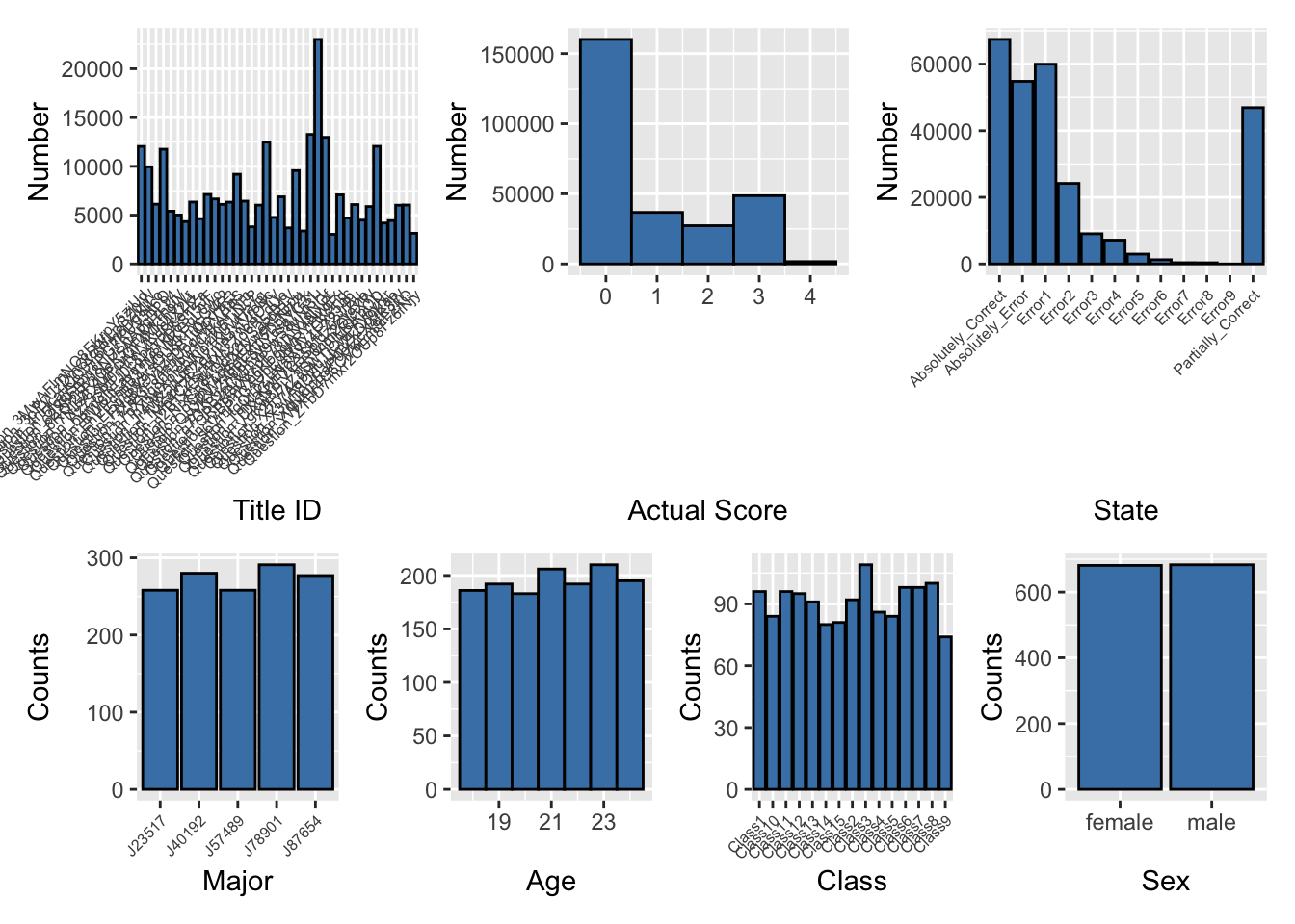
6.2 Pertentage of attempted Knowledge
The plot reveals the distribution of different knowledge areas based on their occurrence percentages. It shows that the knowledge areas are not evenly distributed among the students, with some areas being more prevalent than others.
Click to show code
# Ensure 'knowledge' is a factor
knowledge_expanded$knowledge <- as.factor(knowledge_expanded$knowledge)

# Load necessary libraries
library(ggplot2)
library(dplyr)

# Check the column names in knowledge_expanded
print(colnames(knowledge_expanded))
[1] "title_ID" "student_ID" "class" "time"
[5] "state" "actual_score" "method" "memory"
[9] "timeconsume" "time_change" "sex" "age"
[13] "major" "question_score" "knowledge" "sub_knowledge" # Calculate the count of questions for each knowledge area
knowledge_counts <- knowledge_expanded %>%
group_by(knowledge) %>%
summarise(count = n(), .groups = 'drop')
# Calculate the total number of questions
total_questions <- nrow(knowledge_expanded)
# Calculate the percentage of questions for each knowledge area
knowledge_percentages <- knowledge_counts %>%
mutate(percentage = count / total_questions * 100)
# Add percentage labels to the data frame
knowledge_percentages <- knowledge_percentages %>%
mutate(label = paste0(round(percentage, 1), "%"))
# Reorder knowledge areas by percentage
knowledge_percentages <- knowledge_percentages %>%
arrange(desc(percentage)) %>%
mutate(knowledge = factor(knowledge, levels = knowledge))
# Create a histogram for knowledge percentages with percentage labels
p_knowledge_histogram <- ggplot(knowledge_percentages, aes(x = knowledge, y = percentage, fill = knowledge)) +
geom_bar(stat = "identity", color = 'black') +
labs(title = 'Attempted Percentage of Knowledge Area', x = 'Knowledge Area', y = 'Percentage') +
scale_fill_brewer(palette = "Set3") +
geom_text(aes(label = label), vjust = -0.5, size = 3, color = "black") +
theme_minimal(base_size = 15) +
theme(
axis.text.x = element_text(angle = 45, hjust = 1, size = 10),
axis.title.x = element_text(size = 14, margin = margin(t = 20)),
axis.title.y = element_text(size = 14, margin = margin(r = 20)),
plot.title = element_text(size = 12, face = "bold", margin = margin(b = 20)),
legend.position = "none"
)print(p_knowledge_histogram)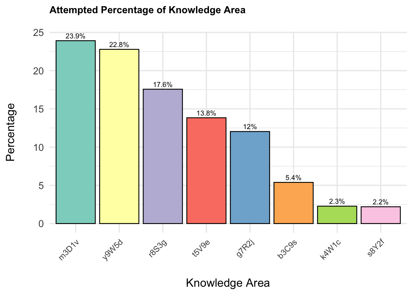
Tip
The least represented knowledge areas are
4W1c(2.3%) and5Y2f(2.2%). These areas show significantly lower representation compared to the major knowledge areas.The higher percentages in certain knowledge areas suggest that students may be more focused or more frequently exposed to these areas.
6.2 Performance by questions
6.2.1 Static heatmap for average max actual score per question (normalised and non normalised)
Click to show code
library(dplyr)
library(ggplot2)
library(plotly)

# Check the column names in knowledge_expanded
print(knowledge_expanded)
# A tibble: 274,490 × 16
title_ID student_ID class time state actual_score method memory timeconsume
<chr> <chr> <chr> <dbl> <chr> <dbl> <chr> <dbl> <dbl>
1 Questio… d554e419f… Clas… 1.70e9 Part… 1 Metho… 196 2
2 Questio… b92448e12… Clas… 1.70e9 Part… 1 Metho… 332 6
3 Questio… 6b22922bf… Clas… 1.70e9 Erro… 0 Metho… 0 2
4 Questio… 72d383f55… Clas… 1.70e9 Part… 1 Metho… 196 3
5 Questio… 3c89c7f1d… Clas… 1.70e9 Erro… 0 Metho… 0 4
6 Questio… f26c1d520… Clas… 1.70e9 Erro… 0 Metho… 0 3
7 Questio… 95i3ttsko… Clas… 1.70e9 Part… 1 Metho… 336 4
8 Questio… c00c91256… Clas… 1.70e9 Abso… 0 Metho… 320 4
9 Questio… 4xh67ezjc… Clas… 1.70e9 Abso… 2 Metho… 324 2
10 Questio… b92448e12… Clas… 1.70e9 Part… 1 Metho… 204 2
# ℹ 274,480 more rows
# ℹ 7 more variables: time_change <dttm>, sex <chr>, age <dbl>, major <chr>,
# question_score <dbl>, knowledge <fct>, sub_knowledge <chr># Ensure 'actual_score' and 'question_score' are numeric
knowledge_expanded <- knowledge_expanded %>%
mutate(actual_score = as.numeric(actual_score),
question_score = as.numeric(question_score))
# Calculate the normalised highest actual_score for each student for each question and knowledge area
highest_scores <- knowledge_expanded %>%
group_by(student_ID, title_ID, knowledge) %>%
summarise(highest_actual_score = max(actual_score, na.rm = TRUE)/question_score, .groups = 'drop')
# Calculate the normalised average highest actual_score for each title_ID and knowledge area
average_highest_scores <- highest_scores %>%
group_by(title_ID, knowledge) %>%
summarise(average_highest_score = mean(highest_actual_score, na.rm = TRUE), .groups = 'drop')
# Retrieve the question_score for each title_ID and knowledge
average_highest_scores <- average_highest_scores %>%
left_join(knowledge_expanded %>% select(title_ID, question_score) %>% distinct(), by = "title_ID")
# Ensure 'knowledge' is treated as a factor for ggplot2 aesthetics
average_highest_scores <- average_highest_scores %>%
mutate(knowledge = as.factor(knowledge))
# Define the color scale limits based on your data range
color_scale_limits <- range(average_highest_scores$average_highest_score, na.rm = TRUE)
# Create the heatmap using ggplot2 with custom hover text
p_heatmap <- ggplot(average_highest_scores, aes(x = knowledge, y = title_ID, fill = average_highest_score,
text = paste("Avg Highest Score:", round(average_highest_score, 2),
"<br>Question Score:", question_score))) +
geom_tile(color = "white") +
scale_fill_gradient2(low = "blue", mid = "green", high = "red", midpoint = 0.9,
limits = color_scale_limits, name = "Avg Highest Score") +
labs(title = "Normalised Average Highest Actual Score per Knowledge Area per Question",
x = "Knowledge Areas",
y = "Question IDs",
fill = "Avg Highest Score") +
theme_minimal(base_size = 15) +
theme(
axis.text.x = element_text(angle = 45, hjust = 1, size = 10),
axis.text.y = element_text(size = 6),
axis.title.x = element_text(size = 10, margin = margin(t = 15)),
axis.title.y = element_text(size = 10, margin = margin(r = 15)),
plot.title = element_text(size = 8, face = "bold", margin = margin(b = 15)),
legend.title = element_text(size = 8), # Adjust legend title size
legend.text = element_text(size = 8), # Adjust legend text size
legend.key.size = unit(1, "cm"), # Adjust size of the legend keys
legend.position = "right"
)
# Convert the ggplot object to a plotly object for interactivity
p_heatmap_interactive1 <- ggplotly(p_heatmap, tooltip = "text")p_heatmap_interactive1 Click to show code
library(dplyr)
library(ggplot2)
library(plotly)

print(knowledge_expanded)
# A tibble: 274,490 × 16
title_ID student_ID class time state actual_score method memory timeconsume
<chr> <chr> <chr> <dbl> <chr> <dbl> <chr> <dbl> <dbl>
1 Questio… d554e419f… Clas… 1.70e9 Part… 1 Metho… 196 2
2 Questio… b92448e12… Clas… 1.70e9 Part… 1 Metho… 332 6
3 Questio… 6b22922bf… Clas… 1.70e9 Erro… 0 Metho… 0 2
4 Questio… 72d383f55… Clas… 1.70e9 Part… 1 Metho… 196 3
5 Questio… 3c89c7f1d… Clas… 1.70e9 Erro… 0 Metho… 0 4
6 Questio… f26c1d520… Clas… 1.70e9 Erro… 0 Metho… 0 3
7 Questio… 95i3ttsko… Clas… 1.70e9 Part… 1 Metho… 336 4
8 Questio… c00c91256… Clas… 1.70e9 Abso… 0 Metho… 320 4
9 Questio… 4xh67ezjc… Clas… 1.70e9 Abso… 2 Metho… 324 2
10 Questio… b92448e12… Clas… 1.70e9 Part… 1 Metho… 204 2
# ℹ 274,480 more rows
# ℹ 7 more variables: time_change <dttm>, sex <chr>, age <dbl>, major <chr>,
# question_score <dbl>, knowledge <fct>, sub_knowledge <chr># Ensure 'actual_score' and 'question_score' are numeric
knowledge_expanded <- knowledge_expanded %>%
mutate(actual_score = as.numeric(actual_score),
question_score = as.numeric(question_score))
# Calculate the highest actual_score for each student for each question and knowledge area
highest_scores <- knowledge_expanded %>%
group_by(student_ID, title_ID, knowledge) %>%
summarise(highest_actual_score = max(actual_score, na.rm = TRUE), .groups = 'drop')
# Calculate the average highest actual_score for each title_ID and knowledge area
average_highest_scores <- highest_scores %>%
group_by(title_ID, knowledge) %>%
summarise(average_highest_score = mean(highest_actual_score, na.rm = TRUE), .groups = 'drop')
# Retrieve the question_score for each title_ID and knowledge
average_highest_scores <- average_highest_scores %>%
left_join(knowledge_expanded %>% select(title_ID, question_score) %>% distinct(), by = "title_ID")
# Ensure 'knowledge' is treated as a factor for ggplot2 aesthetics
average_highest_scores <- average_highest_scores %>%
mutate(knowledge = as.factor(knowledge))
# Define the color scale limits based on your data range
color_scale_limits <- range(average_highest_scores$average_highest_score, na.rm = TRUE)
# Create the heatmap using ggplot2 with custom hover text
p_heatmap <- ggplot(average_highest_scores, aes(x = knowledge, y = title_ID, fill = average_highest_score,
text = paste("Avg Highest Score:", round(average_highest_score, 2),
"<br>Question Score:", question_score))) +
geom_tile(color = "white") +
scale_fill_gradient2(low = "blue", mid = "green", high = "red", midpoint = 2.5,
limits = color_scale_limits, name = "Avg Highest Score") +
labs(title = "Non-normalised Average Highest Actual Score per Knowledge Area per Question",
x = "Knowledge Areas",
y = "Question IDs",
fill = "Avg Highest Score") +
theme_minimal(base_size = 15) +
theme(
axis.text.x = element_text(angle = 45, hjust = 1, size = 10),
axis.text.y = element_text(size = 6),
axis.title.x = element_text(size = 10, margin = margin(t = 15)),
axis.title.y = element_text(size = 10, margin = margin(r = 15)),
plot.title = element_text(size = 8, face = "bold", margin = margin(b = 15)),
legend.title = element_text(size = 8), # Adjust legend title size
legend.text = element_text(size = 8), # Adjust legend text size
legend.key.size = unit(1, "cm"), # Adjust size of the legend keys
legend.position = "right"
)
# Convert the ggplot object to a plotly object for interactivity
p_heatmap_interactive2 <- ggplotly(p_heatmap, tooltip = "text")p_heatmap_interactive2The plot illustrates the average highest scores students achieve across different knowledge areas. In Knowledge Area b3C9s, Question_FNg8X9v5zcbB1tQrxHR3 stands out with a question score of 4, resulting in a more intense color on the plot. Conversely, Knowledge Area r8S3g has questions with a question score of 1, and Knowledge Area t5V9e has questions with a question score of 2. The remaining questions across other knowledge areas generally have a question score of 2.
Although many scores are displayed in shades of green, indicating a similar range of scores, the color intensity variations provide insights into the relative difficulty and performance across different questions.
6.2.2 Static heatmap for Average of methods used per question
Click to show code
library(dplyr)
library(ggplot2)
library(plotly)

# Check the column names in mastery_scores
print(mastery_scores)
# A tibble: 58,510 × 10
# Groups: student_ID, title_ID, knowledge, class [57,151]
student_ID title_ID knowledge class sub_knowledge total_points total_attempts
<chr> <chr> <chr> <chr> <chr> <dbl> <int>
1 0088dc183… Questio… t5V9e Clas… t5V9e_e1k6ci… 1 23
2 0088dc183… Questio… t5V9e Clas… t5V9e_e1k6ci… 1 9
3 0088dc183… Questio… m3D1v Clas… m3D1v_r1d7fr… 4.67 7
4 0088dc183… Questio… g7R2j Clas… g7R2j_e0v1yl… 7.67 22
5 0088dc183… Questio… y9W5d Clas… y9W5d_c0w4mj… 1 1
6 0088dc183… Questio… m3D1v Clas… m3D1v_r1d7fr… 1 1
7 0088dc183… Questio… m3D1v Clas… m3D1v_v3d9is… 1 2
8 0088dc183… Questio… y9W5d Clas… y9W5d_p8g6dg… 1.67 4
9 0088dc183… Questio… r8S3g Clas… r8S3g_n0m9rs… 2 8
10 0088dc183… Questio… y9W5d Clas… y9W5d_e2j7p9… 3.67 11
# ℹ 58,500 more rows
# ℹ 3 more variables: unique_methods <int>, absolutely_correct_methods <int>,
# adjusted_points <dbl># Ensure 'unique_methods' column is numeric if needed
mastery_scores <- mastery_scores %>%
mutate(unique_methods = as.numeric(unique_methods))
# Aggregate data to calculate the average number of unique methods per question and knowledge area
method_counts <- mastery_scores %>%
group_by(student_ID, title_ID, knowledge) %>%
summarise(avg_methods = mean(unique_methods, na.rm = TRUE), .groups = 'drop')
# Further aggregate to get the average number of methods across all students for each title_ID and knowledge
method_counts_summary <- method_counts %>%
group_by(title_ID, knowledge) %>%
summarise(avg_methods = mean(avg_methods, na.rm = TRUE), .groups = 'drop')
# Ensure 'knowledge' is treated as a factor for ggplot2 aesthetics
method_counts_summary <- method_counts_summary %>%
mutate(knowledge = as.factor(knowledge))
# Create the heatmap using ggplot2
p_heatmap <- ggplot(method_counts_summary, aes(x = knowledge, y = title_ID, fill = avg_methods,
text = paste("Knowledge Area:", knowledge,
"<br>Title ID:", title_ID,
"<br>Avg Methods:", round(avg_methods, 2)))) +
geom_tile(color = "white") +
scale_fill_gradient2(low = "white", high = "blue", mid = "green", midpoint = mean(method_counts_summary$avg_methods, na.rm = TRUE), name = "Avg Methods") +
labs(title = "Average Methods used per Knowledge Area per Question",
x = "Knowledge Areas",
y = "Question IDs",
fill = "Avg Methods") +
theme_minimal(base_size = 15) +
theme(
axis.text.x = element_text(angle = 45, hjust = 1, size = 10),
axis.text.y = element_text(size = 8),
axis.title.x = element_text(size = 10, margin = margin(t = 20)),
axis.title.y = element_text(size = 10, margin = margin(r = 20)),
plot.title = element_text(size = 8, face = "bold", margin = margin(b = 20)),
legend.title = element_text(size = 8), # Adjust legend title size
legend.text = element_text(size = 8), # Adjust legend text size
legend.key.size = unit(1, "cm"), # Adjust size of the legend keys
legend.position = "right"
)
# Convert the ggplot object to a plotly object for interactivity
p_heatmap_interactive_method <- ggplotly(p_heatmap, tooltip = "text")p_heatmap_interactive_methodStudents applied more methods in certain knowledge areas, particularly in g7R2j with Question_5fgqjSBwTPG7KUV3it6O, in r8S3g with Question_q7OpB2zCMmW9wS8uNt3H and Question_fZrP3FJ4ebUogW9V7taS, and in t5V9e with Question_3oPyUzDmQtcMfLpGZ0jW and Question_3MwAFlmNO8EKrpY5zjUd. This indicates a higher level of engagement and perhaps complexity in these specific areas and questions.
6.2.3 Static heatmap for Total points per question
Click to show code
library(dplyr)
library(ggplot2)
library(plotly)


# Ensure 'points' is numeric
adjusted_scores <- adjusted_scores %>%
  mutate(points = as.numeric(points))

# Calculate total attempts per question per knowledge area for each student
adjusted_scores <- adjusted_scores %>%
  group_by(student_ID, title_ID, knowledge) %>%
  mutate(attempts = n()) %>%
  ungroup()

# Aggregate data to calculate the total points and total attempts per question and knowledge area for each student
total_points_attempts <- adjusted_scores %>%
  group_by(student_ID, title_ID, knowledge) %>%
  summarise(total_points_sum = sum(points, na.rm = TRUE),
            total_attempts = sum(attempts, na.rm = TRUE), .groups = 'drop')

# Further aggregate to get the total points sum and total attempts across all students for each title_ID and knowledge
total_summary <- total_points_attempts %>%
  group_by(title_ID, knowledge) %>%
  summarise(total_points_sum = sum(total_points_sum, na.rm = TRUE),
            total_attempts = sum(total_attempts, na.rm = TRUE), .groups = 'drop')

# Ensure 'knowledge' is treated as a factor for ggplot2 aesthetics
total_summary <- total_summary %>%
  mutate(knowledge = as.factor(knowledge))

# Define the color scale limits based on your data range
color_scale_limits <- range(total_summary$total_points_sum, na.rm = TRUE)

# Create the heatmap using ggplot2 with custom hover text
p_heatmap <- ggplot(total_summary, aes(x = knowledge, y = title_ID, fill = total_points_sum,
                                       text = paste("Total Points:", total_points_sum, "<br>Total Attempts:", total_attempts))) +
  geom_tile(color = "white") +
  scale_fill_gradient2(low = "blue", mid = "green", high = "red", midpoint = mean(color_scale_limits, na.rm = TRUE),
                       limits = color_scale_limits, name = "Total Points") +
  labs(title = "Total Points per Question per Knowledge Area",
       x = "Knowledge Areas",
       y = "Question IDs",
       fill = "Total Points") +
  theme_minimal(base_size = 15) +
  theme(
    axis.text.x = element_text(angle = 45, hjust = 1, size = 10),
    axis.text.y = element_text(size = 6),
    axis.title.x = element_text(size = 10, margin = margin(t = 15)),
    axis.title.y = element_text(size = 10, margin = margin(r = 15)),
    plot.title = element_text(size = 8, face = "bold", margin = margin(b = 15)),
    legend.title = element_text(size = 8),  # Adjust legend title size
    legend.text = element_text(size = 8),  # Adjust legend text size
    legend.key.size = unit(1, "cm"),        # Adjust size of the legend keys
    legend.position = "right"
  )

# Convert the ggplot object to a plotly object for interactivity
p_heatmap_interactive <- ggplotly(p_heatmap, tooltip = "text")
# Print the interactive heatmap
p_heatmap_interactiveBased on the point system, there are notable concentrations of total points in various knowledge areas. High Total Points Concentration is observed in the g7R2j knowledge area, particularly for Question_5fgqjSBwTPG7KUV3it6O, which has the highest total points indicated by the darker blue color. This suggests that a significant number of students attempted this question and scored well. Following closely is the t5V9e knowledge area with Question_3MwAFlmNO8EKrpY5zjUd, which has the second highest total points. Middle Points Concentration is seen in several knowledge areas:
In
r8S3gwith Question_q7OpB2zCMmW9wS8uNt3H.In
m3D1vwith Questions_QRm48lXxzdP7Tn1WgNOf and Question_4nHcauCQ0Y6Pm8DgKlLo.In
y9W5dwith Questions_QRm48lXxzdP7Tn1WgNOf, Question_Az73sM0rHfWVKuc4X2kL, and Question_EhVPdmlB31M8WKGqL0wc.
Low Points Concentration is observed in the r8S3g and m3D1v knowledge areas, indicating that these areas may be more challenging for students or less frequently attempted.
6.3 Performance by knowledge
6.3.1 Ridge plot for sum(max actual score per qns) for 8 knowledge normalised
Click to show code
# Load the necessary library
library(dplyr)

# Group by 'title_ID', 'student_ID', and 'knowledge' and find the max 'actual_score' for each group
max_scores <- adjusted_scores %>%
  group_by(title_ID, student_ID, knowledge) %>%
  summarize(max_actual_score = max(actual_score, na.rm = TRUE))

# Display the result
print(max_scores)
# A tibble: 57,151 × 4
# Groups: title_ID, student_ID [50,482]
title_ID student_ID knowledge max_actual_score
<chr> <chr> <chr> <dbl>
1 Question_3MwAFlmNO8EKrpY5zjUd 0088dc183f73c83f763e t5V9e 2
2 Question_3MwAFlmNO8EKrpY5zjUd 00cbf05221bb479e66c3 t5V9e 2
3 Question_3MwAFlmNO8EKrpY5zjUd 00df647ee4bf7173642f t5V9e 2
4 Question_3MwAFlmNO8EKrpY5zjUd 0107f72b66cbd1a0926d t5V9e 2
5 Question_3MwAFlmNO8EKrpY5zjUd 011d454f199c123d44ad t5V9e 2
6 Question_3MwAFlmNO8EKrpY5zjUd 01558eef77a8d39b7103 t5V9e 2
7 Question_3MwAFlmNO8EKrpY5zjUd 016226278e6a69e10aa4 t5V9e 2
8 Question_3MwAFlmNO8EKrpY5zjUd 01a691413dc5897db83f t5V9e 2
9 Question_3MwAFlmNO8EKrpY5zjUd 01d8aa21ef476b66c573 t5V9e 2
10 Question_3MwAFlmNO8EKrpY5zjUd 01qkq6w2v62cimidb3b7 t5V9e 2
# ℹ 57,141 more rows# Load the necessary libraries
library(dplyr)
library(ggplot2)
library(ggridges)
library(viridis) # For the viridis color palette
# Assuming your dataframe is named adjusted_score
# and it has columns 'title_ID', 'student_ID', 'knowledge', and 'actual_score'
# Group by 'title_ID', 'student_ID', and 'knowledge' and find the max 'actual_score' for each group
max_scores <- adjusted_scores %>%
group_by(title_ID, student_ID, knowledge) %>%
summarize(max_actual_score = max(actual_score, na.rm = TRUE), .groups = 'drop')
# Check the aggregated data
print(head(max_scores))# A tibble: 6 × 4
title_ID student_ID knowledge max_actual_score
<chr> <chr> <chr> <dbl>
1 Question_3MwAFlmNO8EKrpY5zjUd 0088dc183f73c83f763e t5V9e 2
2 Question_3MwAFlmNO8EKrpY5zjUd 00cbf05221bb479e66c3 t5V9e 2
3 Question_3MwAFlmNO8EKrpY5zjUd 00df647ee4bf7173642f t5V9e 2
4 Question_3MwAFlmNO8EKrpY5zjUd 0107f72b66cbd1a0926d t5V9e 2
5 Question_3MwAFlmNO8EKrpY5zjUd 011d454f199c123d44ad t5V9e 2
6 Question_3MwAFlmNO8EKrpY5zjUd 01558eef77a8d39b7103 t5V9e 2# Create the ridge plot with quantiles and quartiles
p_ridge_max_scores_quantiles <- ggplot(max_scores, aes(x = max_actual_score, y = knowledge, fill = factor(stat(quantile)))) +
stat_density_ridges(
geom = "density_ridges_gradient",
calc_ecdf = TRUE,
quantiles = 4,
quantile_lines = TRUE
) +
scale_fill_viridis_d(name = "Quartiles") +
labs(title = "Max Actual Scores Distribution per Knowledge Area", x = "Max Actual Score", y = "Knowledge Area") +
theme_ridges() +
theme(
axis.text.y = element_text(size = 8),
axis.title.x = element_text(size = 10, margin = margin(t = 10), hjust = 0.5),
axis.title.y = element_text(size = 10, margin = margin(r = 10), hjust = 0.5),
plot.title = element_text(size = 10, face = "bold", margin = margin(b = 20)),
legend.position = "right",
legend.title = element_text(size = 8), # Customize the legend title font
legend.text = element_text(size = 8
))# Print the ridge plot
print(p_ridge_max_scores_quantiles)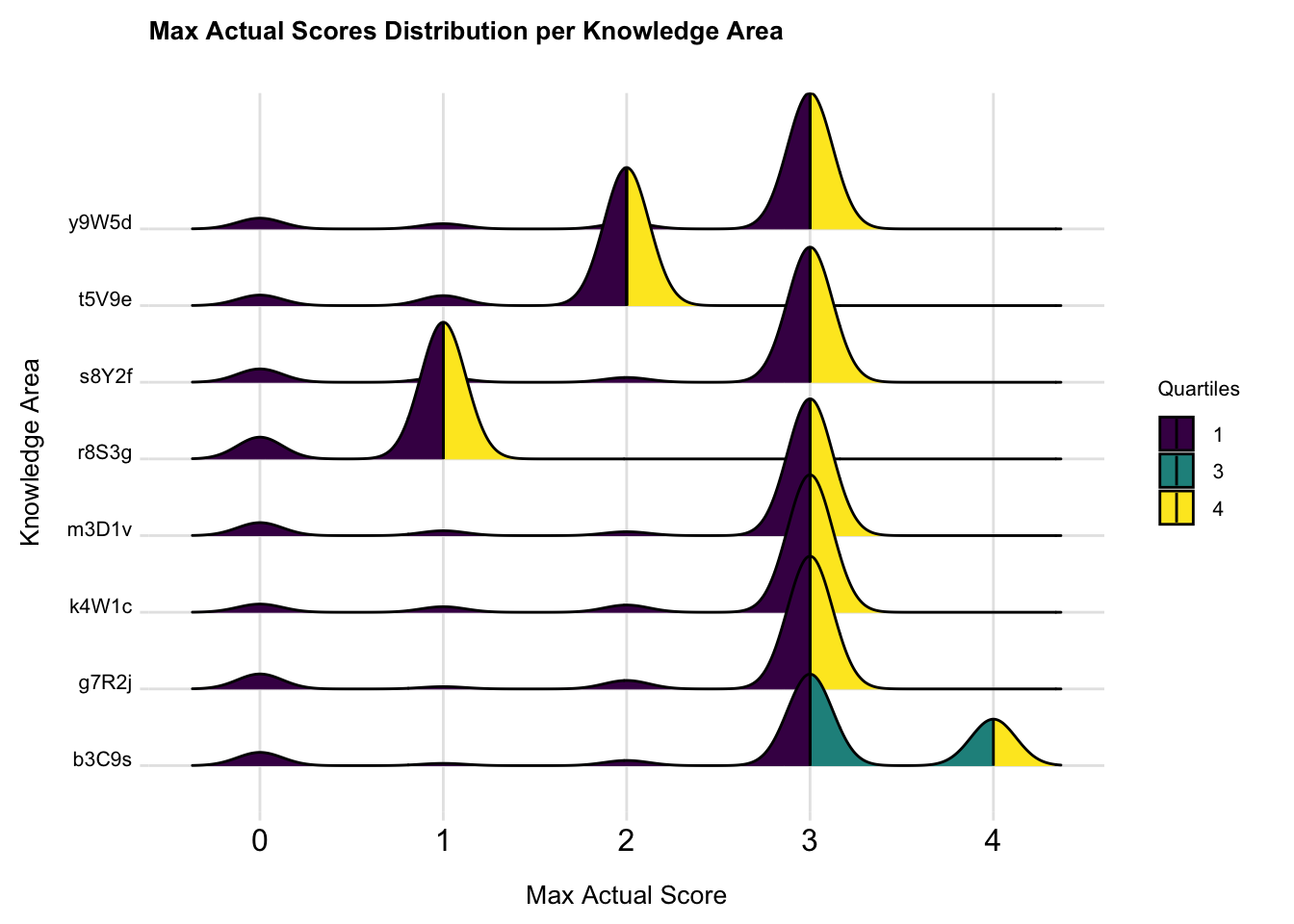
From the plot, we can observe distinct patterns in score distribution across different knowledge areas. Knowledge areas with prominent yellow sections indicate that students performed well in these areas.Areas with more purple suggest lower student performance, we can tell the performance of students getting highest score on the knowledge y9W5d, s8Y2f, m3D1v, k4W1c and g7R2j are quite similar. R8S3g has more students get score of 0. Areas with a wider distribution of colors and less sharp peaks, indicate more variability in student performance, such as knowledge b3C9s
6.3.2 Distribution of Total Mastery Points by Knowledge
Click to show code
library(dplyr)
library(ggplot2)

# Assuming your dataframe is named knowledge_mastery and it has columns 'knowledge' and 'total_score'

# Calculate the mean total score for each knowledge area
mean_scores <- knowledge_mastery %>%
  group_by(knowledge) %>%
  summarize(mean_total_score = mean(total_score, na.rm = TRUE)) %>%
  arrange(desc(mean_total_score))

# Reorder the factor levels of knowledge based on the mean total scores
knowledge_mastery <- knowledge_mastery %>%
  mutate(knowledge = factor(knowledge, levels = mean_scores$knowledge))

# Create the ggplot2 boxplot with uniform color, ordered by mean total score
p <- ggplot(knowledge_mastery, aes(x = knowledge, y = total_score)) +
  geom_boxplot(fill = "gray", color = "darkblue", alpha = 0.7) +
  geom_jitter(width = 0.2, alpha = 0.5, color = "skyblue") +  # Adding jitter for individual points
  theme_minimal() +
  labs(
    title = "Distribution of Total Mastery Points by Knowledge",
    x = "Knowledge",
    y = "Total Mastery Points"
  ) +
  theme(
    axis.text.x = element_text(angle = 45, hjust = 1)
  )
# Print the boxplot
print(p)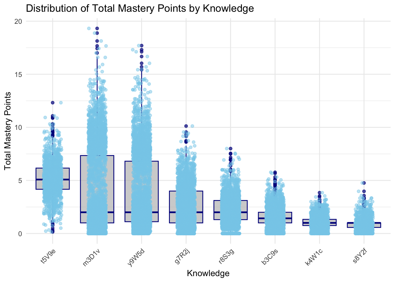
::: {.callout-tip appearance=“simple”} The knowledge areas m3D1v, y9W5d, and t5V9e demonstrate the highest median total mastery points, reflecting strong student performance and effective teaching methods. In contrast, k4W1c, b3C9s, and s8Y2f exhibit the lowest median scores, indicating these areas are more challenging for students and may require targeted interventions. Additionally, knowledge areas such as t5V9e and g7R2j show moderate performance, suggesting a fair understanding but highlighting opportunities for further improvement.
:::
Click to show code
library(dplyr)
library(ggplot2)

# Assuming your dataframe is named knowledge_mastery and it has columns 'sub_knowledge' and 'total_score'

# Calculate the mean total score for each sub_knowledge area
mean_scores <- knowledge_mastery %>%
  group_by(sub_knowledge) %>%
  summarize(mean_total_score = mean(total_score, na.rm = TRUE)) %>%
  arrange(desc(mean_total_score))

# Reorder the factor levels of sub_knowledge based on the mean total scores
knowledge_mastery <- knowledge_mastery %>%
  mutate(sub_knowledge = factor(sub_knowledge, levels = mean_scores$sub_knowledge))

# Create the ggplot2 boxplot with uniform color, ordered by mean total score
p <- ggplot(knowledge_mastery, aes(x = sub_knowledge, y = total_score)) +
  geom_boxplot(fill = "gray", color = "darkblue", alpha = 0.7) +
  geom_jitter(width = 0.2, alpha = 0.5, color = "skyblue") +  # Adding jitter for individual points
  theme_minimal() +
  labs(
    title = "Distribution of Total Mastery Points by Sub-Knowledge",
    x = "Sub-Knowledge",
    y = "Total Mastery Points"
  ) +
  theme(
    axis.text.x = element_text(angle = 45, hjust = 1)
  )
# Print the boxplot
print(p)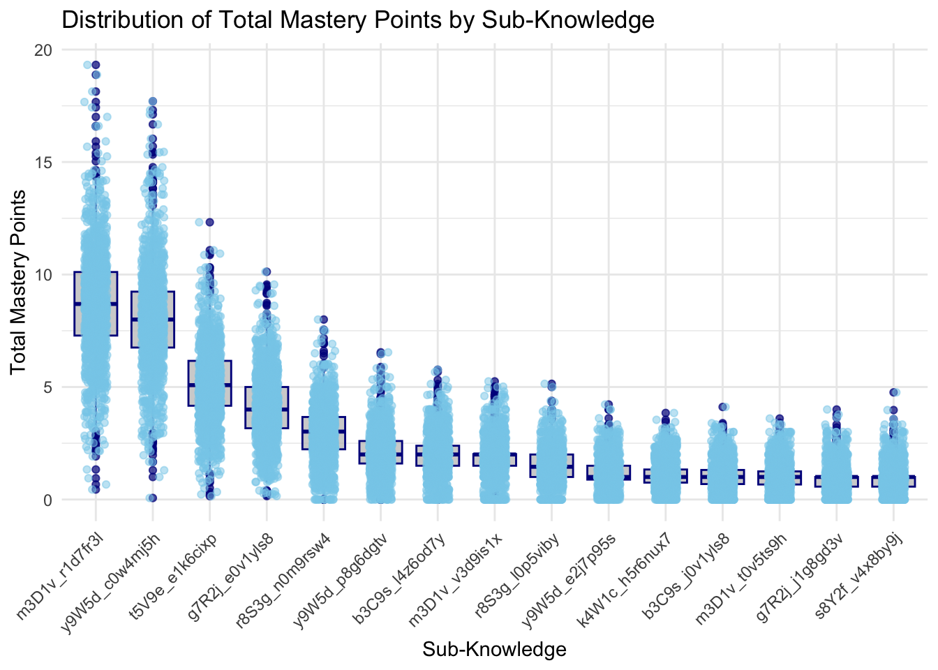
The boxplots provide a comprehensive view of the distribution of total mastery points across different knowledge and sub-knowledge areas. In the first plot, which shows the distribution of total mastery points by knowledge, there is significant variation in scores across the different knowledge areas. For instance, knowledge areas like y9W5d, m3D1v, have higher maximum scores, with some students achieving mastery points close to 20. This indicates that these areas are well-understood by many students. Conversely, areas such as K4W1c and s8Y2f show lower median scores and fewer high outliers, suggesting these might be less well-mastered or less attempted by students.
The second plot breaks down the performance further by sub-knowledge areas. This detailed view shows how students perform on specific topics within each broader knowledge area. High-performing sub-knowledge areas, such as m3D1v_r1d7f3j, y9W5d_q0w4mj5h, and t5V9e_e1k6cixp, mirror their parent knowledge areas in achieving high maximum scores. In contrast, sub-knowledge areas like s8Y2f_v4x8b9vj and g7R2j_j1g8g3v have lower overall scores, indicating these topics might need more attention in teaching or resources. The plots also highlight consistency in scores.
7. Conclusion
In summary, the high mastery knowledge areas identified are y9W5d, m3D1v, t5V9e, and g7R2j. These areas have shown higher maximum scores and mastery points, indicating good student understanding and performance. Within these knowledge areas, specific sub-knowledge topics such as y9W5d_q0w4mj5h, m3D1v_r1d7f3j, and t5V9e_e1k6cixp are particularly well-mastered, reflecting students’ strong grasp of these topics. In contrast, sub-knowledge areas like s8Y2f_v4x8by9j and g7R2j_j1g8g3v show lower overall scores, indicating these topics are not well mastered by students and may require additional attention in teaching or resources.